


How to use VLookUp Function
- Mar 26, 2016
- 2 min read
Updated: Feb 13, 2020
The most common need while using MS Excel is to find a value from a list of items. Here is where the Vlookup function comes handy!

You have a list of employee Numbers of all salespeople in your company and you would like to know how much sales each of the salesperson has made so that you can decide if he/she is eligible for the sales incentive or not.

If you have only a few salespeople, then you can manually look at each salesperson's sale amount and note down the same. However, most companies have many salespeople spread across many regions and this will consume a lot of time if you have to check everyone's sales amount manually.
In this case, Vlookup function of Excel is very useful. The Syntax of this is as follows:
=Vlookup(LookupValue, TableArray, ColumnNumber, [TypeOfMatchFlag])
LookupValue = (required Field) This is the item that you want to look up in the table. This must be the first column of the TableArray. In the above example, this is the
TableArray = (required Field) This is the table from which you want to look up the value. This must be the first column of the TableArray.
Column Number = (required Field) This is the column number of the value that you want to be returned in the result. The starting column in the TableArray will be counted as 1, the next column as 2 and so on.
LookupValue = (Optional Field) This is an optional field. This specifies whether you want the Vlookup to find an exact match or an approximate match.
1 or TRUE = This matches the value approximately. In this case, it assumes that the first column is sorted Alphabetically or Numerically and will look for the first approximate match.
0 or FALSE or BLANK = This matches the value exactly. If no exact match is found (even due to minor difference in spelling or blank spaces), this will return an error.
The Sales data is in the following file with the format as shown below :

So you will use the Vlookup() functions as follows on Cell B2 :
=VLOOKUP(A2,[SalesData.xlsx]Sheet1!$B$2:$H$5,7,0)
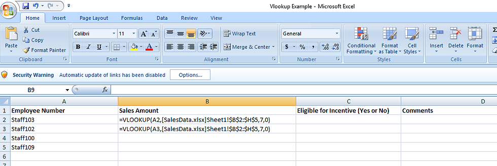
Then you can drag down the formula to the bottom of the list till Cell B5. The results will be dsiplayed as shown below :
This will display the sales amount by each salesperson. Now you can decide if he/she is eligible for the sales incentive or not.
We can use other functions like IF() or other conditions to determine if the salesperson is eligible for incentive or not. This will be covered in a separate post. Till then practise vlookup on a few other lists.
TIPS:
Please note that this function is used to lookup a value when your source table is arranged vertically in many rows. If your table is arranged Horizontally in many columns, then you will have to use a different function called HLOOKUP().
This function can be used to compare two lists to check which items are available in the second list and which are not.


Comments